Copyright © 2004 Samuel L. Baker
Revised December 2011
CPM can help you figure out:
This document describes the steps for doing CPM analysis for this course. The steps will be illustrated by two examples. I recommend that you work through the examples, so that you can follow the steps yourself when you do the homework.
Example 2 is especially valuable for you to work through. Excel has bugs that vary from version to version. By working through Example 2, and comparing what you get with what I got, you can find out which bugs apply to you and how to work around them when you do the assignment.
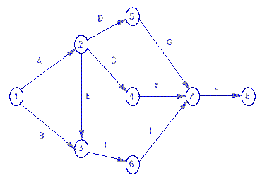
Here's the example:
| Activity | Description | Required Predecessor | Duration |
| A | Product design | (None) | 5 months |
| B | Market research | (None) | 1 |
| C | Production analysis | A | 2 |
| D | Product model | A | 3 |
| E | Sales brochure | A | 2 |
| F | Cost analysis | C | 3 |
| G | Product testing | D | 4 |
| H | Sales training | B, E | 2 |
| I | Pricing | H | 1 |
| J | Project report | F, G, I | 1 |

Some conventions about how to draw these diagrams:
In this example, A and B are the two activities that have no precedessor. They are represented as arrows leading away from node 1.
J is the one activity that has no successor, in this example. It therefore points to the last node, which is node 8. If there were more than one activity with successor, all of those activities' arrows point to the highest number node.
Students sometimes make the mistake of creating a diagram with several starting or ending nodes. Don't do this.
The trickiest part for me of building the above diagram was figuring what to do with activity H. I had drawn an arrow for activity B coming off node 1 and going to mode 3. I had later drawn an arrow for activity E coming off node 2 and going to node 6. Since H requires both B and E, I had to erase my first E arrow and redraw it so it pointed to the same node 3 that B did. H then comes off of node 3 and goes to node 6.
When designing these diagrams, work in pencil.
Start up a new blank spreadsheet. If you are viewing this document on the web, minimize your browser window and then start Excel. That way you can switch from one to the other by pressing Alt+Tab.
In a blank spreadsheet, type the word "Activities" in cell A1. In row 2, type the names of the activities, or their letters. (To make my spreadsheet screen shots fit better on these pages, I set the column widths to 4. You do not have to do this.)

In row 3, type "Nodes". In row 4, type in each activity's start node -- where the tail of its arrow is. Below that, in row 5, type each activity's end node -- where the head of its arrow is. Do this carefully. Mistakes here mess up everything that follows.
To the right, in K2 and K3, type the words "Start" and "End" to label those rows.

In cell A6, type "Times". In row 7, type the time each activity
takes.
Then, select the range of cells containing the node numbers

and copy it to the clipboard.
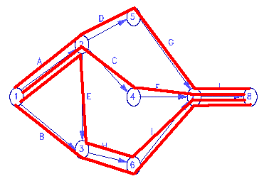
To use Pathfind now, go to Pathfind.
Pathfind is a Java applet that runs inside your browser. When Pathfind is loaded:
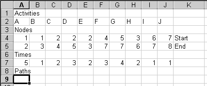
Paste to that cell, to see this:
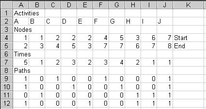
The pasted cells are all 0's and 1's. Each row represents a path. The 1's indicate which activities are in that particular path. For example, row 9 (cells A9:J9) has 1's under activities A, C, F, and J. This says that this path includes activities A, C, F, and J. This corresponds to the path through the middle of the diagram that goes: 1 -A-> 2 -C-> 4 -F-> 7 -J-> 8.
The diagram above shows four paths from node 1 to node 8. Sure enough, Pathfind gives you four rows of 0's and 1's, one row for each path.
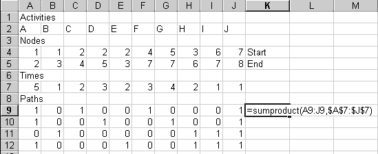
When you enter the formula, the number 11 should appear in K9. That's the time it would take to complete activities A, C, F, and J. You can verify that A takes 5 months, C takes 2, F takes 3, and J takes 1, for a total of 11.
(If you are doing a CPM problem of your own, modify the formula so that the ranges cover the columns you actually have. This advice applies to all the formulas which follow.)
To fill in the other paths' times, copy cell K9, then paste it to K9:K12. The $ signs in the formula see to it that each path's 1's are multiplied by the corresponding numbers in row 7.
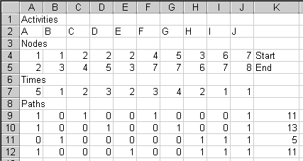
The 1's in row 10 tell us that the critical path is 1 -A-> 2 -D-> 4 -G-> 7 -J-> 8. As managers, we must be sure that activities A, D, G, and J are done on time. If any of those activities is late, the project will be late.
Other paths are not critical because they can waste some time without slowing the project. For example, activity C, in row 9's path, can take up to two extra months and not hold up the project.
To make it easier to see what activities are in each path, go to
cell
A14. Type =if(A9=1,A$2,"") there.
The letter A should appear in cell A14.
This =if(A9=1,A$2,"") function works this way: Inside the parentheses are three expressions separated by commas. The first expression (A9=1) is something that can be either true or false. If the expression is true, the second expression (A$2) is shown in the cell. Otherwise, the third expression ("") is shown in the cell.
In A14, the expression A9=1 is true, so the cell shows what is in A2, which is the letter "A". If A9 had not contained a 1, the A14 would have shown a blank, which is what "" means.
Copy A14 to the clipboard. Then, starting in A14, select a range of cells that goes over to column J and down four rows. The selected range should be the same size as the space that the paths' 1's and 0's take up.
Paste. You should get this:
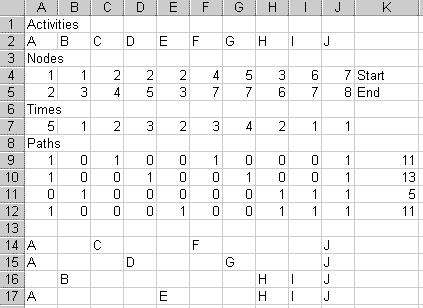
Now you can see which activities are in each path. If your results do not look like the above, make sure that there is one $ in your formula, and that it's in front of the 2 and not in front of the A.
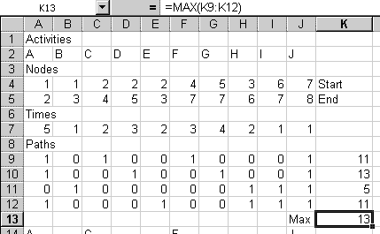
Go to cell J13 and type "Max". Then go to cell K13. Type =MAX(K9:K12) to display the longest path time.
Move to cell K14 and type =IF(K9=K$13,"Critical","")
there.
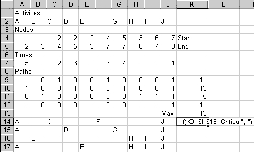
This will put the word "Critical" next to a path whose time equals
the maximum of all the path times. Otherwise, it will put in a blank,
as
it does here, because the 11 in K9 does not equal the 13 in K13.
Copy K14 to the clipboard. (It will seem strange to copy what
appears
to be an empty cell, but do it anyway.) Select cells K14 to K17, and
paste.
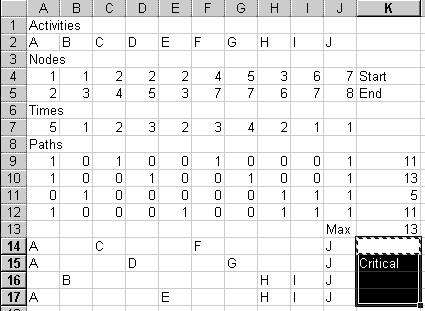
You're done! You've found the time the project will take, and you have identified the critical path, which tells you which activities must be done on time to make the project finish in the least time.
Take a moment to admire your work before plunging in to Example 2.
| Activity | Required Predecessor | Normal Time | Normal Cost | Crash Time | Crash Cost |
| A | (None) | 3 weeks | $3000 | 2 weeks | $5000 |
| B | (None) | 4 | $4000 | 2 | $6000 |
| C | (None) | 5 | $5000 | 3 | $8000 |
| D | A | 8 | $5000 | 6 | $6000 |
| E | A,B | 3 | $3000 | 2 | $4000 |
| F | C | 5 | $4000 | 3 | $8000 |
To start the network diagram, we notice that A, B, and C are the three activities with no
predecessor. They all come off of node 1. A can go node 1 to node 2.
B can go from node 1 to node 3.
C also starts at node 1. D requires A, so D starts at node 2. Here's what we have so far:
Now for activity E. Activity E requires a special trick. The problem is where E should start. E requires A and B. A ends at node 2 and B ends at node 3. E is not allowed to start from both nodes 2 and 3. Activities can have only one start node and only one end node.
What do we do about E? You might consider connecting both A and B to node 2, but that would mess up Activity D. If both A and B were to run from node 1 to node 2 and D came off of node 2, that would be saying that D requires B as well as A. D is supposed to require A, not also B.
Here is the solution:
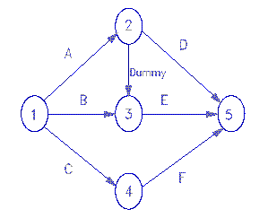
The solution is to add a dummy activity that runs from node 2 to node 3, as shown in the diagram. Then start E at node 3.
If E starts at node 3, it means that E requires B and the dummy activity, the two activities that come in to node 3. The dummy activity, because it starts at node 2, requires A. This makes E require B and A. That is what we want! Meantime, D starts at node 2, so D only requires A. All the requirements are satisfied!
Dummies activities add nothing to the time or the cost. Their purpose is to allow you to represent complex relationships among activities.
These instructions will create the spreadsheet from scratch. Adapting the spreadsheet from example 1 is possible, but tricky, because example 2 has fewer columns and more rows than example 1.If you start with a blank spreadsheet, move the cell selector to A1 and type "Activities". In row 2, type the activities' letters or names. Put the Dummy at the right end of row 2, for two reasons:

Type "Times" in cell A6.
In row 7, type each activity's normal time. The dummy's time is 0.
In row 8, type each activity's crash time. The dummy's crash time is
0.
Copy row 7 and paste it into row 9. Row 9 will be the variable cells when we do the optimization later. Be sure to copy the numbers themselves from row 7 to row 9. Don't put a formula like =A7 in A9.
Label each of the Times rows by typing "Normal" in H7, "Crash" in
H8,
and "Actual" in H9.
(Note: When you do the homework, your number of columns will be
different.
These labels go in the column to the right of the last activity's
information.
Whatever column that is, use its letter in place of "H" in all the
following
instructions and formulas.)
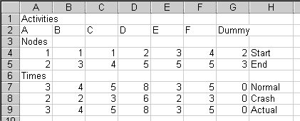
When we do the optimization, we'll set a maximum time for the project and tell the spreadsheet to find the combination of numbers in row 9 that completes the project within that time for the lowest possible cost.
To do that, we need the costs. In cell A10, type "Costs".
In row 11, put each activity's normal cost. In H11, type "Normal".
In row 12, put each activity's crash cost. In H12, type "Crash".
In H13, type "Actual".
Type "0" in G13 for the Dummy's actual cost.
(When you do the homework, your column letters will differ.)
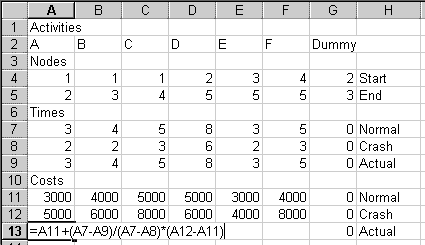
The diagram above also shows a formula we'll put in A13.
Row 13 will have formulas to calculate the actual cost for each activity. Each activity's actual cost depends on how much it is sped up, or "crashed." We assume a linear relationship between speed-up and cost. So, for example, if Activity A can be shortened by 2 weeks at an added cost of $2000, we assume that it can be shortened by 1 week for an added cost of $1000.
The formula to implement this goes first A13. Here it is:
=A11+(A7-A9)/(A7-A8)*(A12-A11)
If you are viewing this in a web browser, you can select and copy the above formula right off of the screen. Then paste it into cell A13 of your spreadsheet.
The logic of the formula:
(A7-A9) is the difference between the normal time and the actual time we use for activity A. This difference is how much time we are saving by speeding up activity A.
(A7-A8) is the difference between the normal time and the crash time. This is the most time we could save by speeding up activity A.
(A7-A9)/(A7-A8) is how much time we are actually saving, as a fraction of how much time we could save, for activity A. In other words, it is the proportion of the possible time savings that we are actually using.
(A12-A11) is the difference between the crash cost and the normal cost
for activity A. This difference is how much cost would go up if we
shortened activity A's time as much as possible.
Multiplying these, to get (A7-A9)/(A7-A8)*(A12-A11), tells us
additional
cost we are incurring by shortening activity A's time from its normal
time
to the actual time we chose. This embodies the linearity assumption -- that if we go part way between the normal time and the crash time, our cost will be that same part way between the normal cost and the crash cost.
The full formula, A11+(A7-A9)/(A7-A8)*(A12-A11), adds that additional cost to A11, the cost of doing the activity in
normal time. This gives us the cost of doing activity A in the amount of time in A9.
Thank you, Dawid from Poland, for writing me about this.
Once that formula is in, copy cell A13 to the clipboard. Select cells A13:F13, and paste.
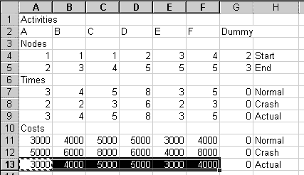
Right now, it may look like the formula isn't doing much, because the Actual costs match the Normal costs. This is because the Actual times match the Normal times. Later, when we shorten the project, this will change.
Now, select the range of node numbers, being sure to include the
dummy activity's node numbers.

Copy this range to the clipboard.
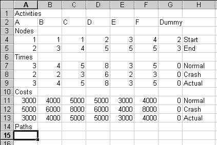
Paste to that cell, to see this:
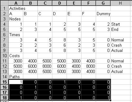
As with the first example, each row represents a path. The 1's indicate which activities are in that particular path. For example, row 15 has 1's under activities A and D. This represents the path 1 -A-> 2 -D-> 5 at the top of the diagram. There are four possible paths from node 1 to node 5, so you have four rows of 0's and 1's.
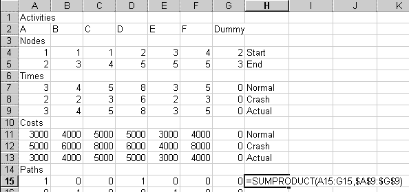
Copy that cell and paste it to H15:H18. (When you do the homework, you will paste to a different range of cells. You will have a different number of actvities and a different number of paths.)
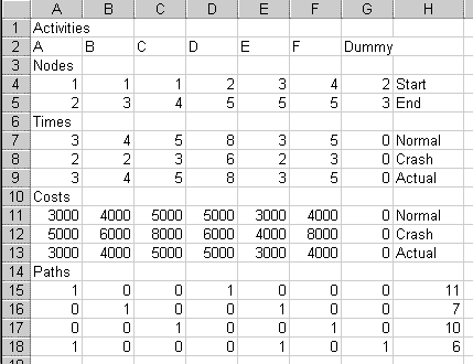
We can now see how long each path takes.
To make it easier to see which activities are in each path, go to cell A20 and type =if(A15=1,A$2,"") (Notice that the $ sign is before the 2, not before the A.) This should put an "A" in A20.
Copy cell A20 to the clipboard. Select the range A20:G23. Paste.
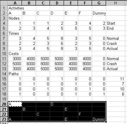
You now should have four rows showing the letters of the activities
that are in each path.
Go back up to cell G19 and type "Max". Go to cell H19 and type =max(H15:H18) This shows how long the slowest path takes.
Go down to cell H20. Put in =IF(H15=H$19,"Critical",""). In this example, "Critical" appears in cell H15, because this first path is the critical path. (In your homework, if the first path does not happen to be critical, this cell will appear blank.)
Copy cell H20. Highlight H20:H23. Paste.
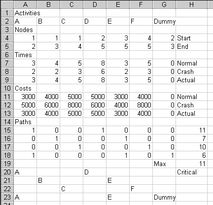
Sure enough, the first path with activities A and D, is the only one
labelled "Critical".
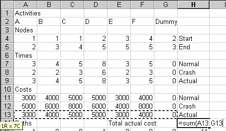
When you complete the formula, you'll see that if we use all normal
times for all activities, the total cost is $24,000.
Fill in the Solver Parameters box as shown here. (For the
homework,
modify the formulas so they cover the rows and columns that you have.)
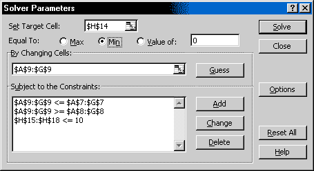
If you are using Excel 2010, choose the Simplex LP method for solution.
If you are using Excel 2000 or earlier, click on Options. Click the checkbox for
assuming a linear model.
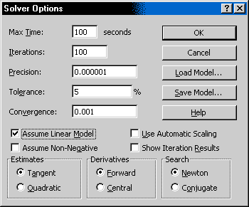
Excel 2007 and 2003 do not need this, but Excel 2000 seems to. If you do not check this box,
Excel 2000 may tell you at some point that there is not a feasible
solution when
actually there is one. Some older Excel versions, though,
give wrong answers if you check this box. For older versions of Excel, my advice is to
first try telling it that this is a linear model, as shown
here,
and see what happens when you Solve.
If it won't give you a solution, uncheck the linear model checkbox and
solve again.
Click on OK in the Solver Options dialog box. Click on Solve in the Solver Parameters dialog box.
If an error message appears, bring back up the Solver Parameters dialog box.
Bug workaround: If you get a message that there is no feasible solution, try changing the Assume Linear Model option. That is, click Solver's Options button, then check Assume Linear Model if it's unchecked, or uncheck it if it's checked.
If you still get the no-feasible-solution message, change the Solver Parameters as shown here to exclude the dummy
activity from the Changing Cells and the Constraints.
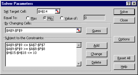
The ranges for the Changing Cells and the Constraints stop at column
F. Column G has the dummy activity.
Excel 2000 and later should not require this modification.
Please if you have
to resort to this.
Another bug workaround: If the word "Critical" does not appear everywhere that it should, Solve a second time. Just bring up Solver and click the Solve button again.
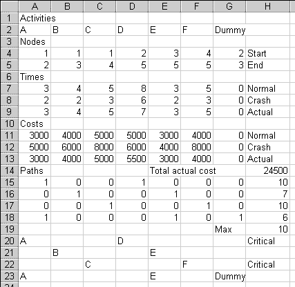
To get finished in 10 weeks (H19 now has 10), we'll have to spend $24,500 (H14 now has 24500).
As manager, you'll be busier. You now have two critical paths to worry about, 1 -A-> 2 -D-> 5, and 1 -C-> 4 -F-> 5. If any of the four activites in those paths is late, the project will take more than 10 weeks.
Let's add three more rows, to make it easier to see which activities have speeded up and at what extra cost:
Go to cell A24 and type "Crashed by how much"
Then go to A25 and put =A7-A9 there. This is the Actual time
minus the Normal time.
Go to cell A26. Type in =A13-A11. This is the difference
between
the current Actual cost and the Normal cost.
Select A25:A26. Copy to the clipboard. Select A25:F25, and paste.
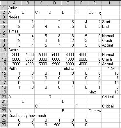
We see that Activity D has been shortened by 1 week, at an extra cost of $500.
Here are our results so far. An explanation follows:
| Weeks | Project cost | Penalty cost | Total cost |
| 11 | $24,000 | $7,500 | $31,500 |
| 10 | 24,500 | 5,000 | 29,500 |
If we use normal times, the project takes 11 weeks, which runs over the schedule by 3 weeks. We lose $7500 in penalties. The total project cost is $24,000 + $7,500 = $31,500.
If we crash by 1 week, the project takes 10 weeks. Our penalty cost is $5,000. Direct project cost is $24,500, as we just saw. The total is $29,500. This is less than $31,500, so ten weeks is better than eleven weeks.
To try getting done in 9 weeks, go back to the Solver (step 9). Change the H15:H18 <= 10 constraint to H15:H18 <= 9. Solve. The cost rises to $26,500. The penalty for being one week late is $2,500. Total cost is $26,500 + $2,500 = $29,000. This is less than $29,500, so nine weeks is better than ten weeks.
| Weeks | Project cost | Penalty cost | Total cost |
| 11 | $24,000 | $7,500 | $31,500 |
| 10 | 24,500 | 5,000 | 29,500 |
| 9 | 26,500 | 2,500 | 29,000 |
Notice that cutting the second week added more to cost (second column) than cutting the first week. Cutting one week increased project cost by $500. Cutting the second week increased project cost by $2000, from $24,500 to $26,500. The law of diminishing returns is at work here.
Should we save three weeks and be on time? To try getting done in 8 weeks, go back to the Solver. Change the H15:H18 <= 9 constraint to H15:H18 <= 8. Solve. You should find that the cost is $30,000. There is no penalty, but $30,000 is more than $29,500, so we lose money by being on time. We are better off being one week late and paying the penalty.
What about saving four weeks and being early? Thanks to the law of diminishing returns, we don't need to consider shorter project durations than 8 weeks. Going from 9 weeks to 8 added $3,500 to cost. The law of diminishing returns implies that going from 8 weeks to 7 will add at least $3,500 more to cost. That is more than the $1000 bonus, so we know 7 weeks is a loser.
If the bonus is linear (in other words, if we get the same bonus for each additional week that we are early) then the law of diminishing returns implies that we can stop our analysis as soon as the total cost, including the bonus, starts to rise.
Here is the whole table. The bonus
for being early is treated as a negative penalty.
| Weeks | Project cost | Penalty cost | Total cost |
| 11 | $24,000 | $7,500 | $31,500 |
| 10 | 24,500 | 5,000 | 29,500 |
| 9 | 26,500 | 2,500 | 29,000 |
| 8 | 30,000 | 0 | 30,000 |
| 7 | Don't bother | -1000 | will be higher |
We conclude that our optimal production schedule is 9 weeks. It has the least total cost.
| Activity | Required Predecessor | Normal Time | Normal Cost | Crash Time | Crash Cost |
| A | (None) | 4 | $2000 | 3 | $2600 |
| B | (None) | 6 | 3000 | 3 | 9000 |
| C | (None) | 4 | 8000 | 2 | 12000 |
| D | A | 8 | 4500 | 5 | 9000 |
| E | C | 6 | 6000 | 4 | 8000 |
| F | A | 5 | 3000 | 3 | 6000 |
| G | C | 9 | 6000 | 4 | 10000 |
| H | B, D, E | 4 | 1800 | 3 | 2000 |
| I | B, D, E | 6 | 1000 | 5 | 1200 |
| J | B, D, E | 7 | 2000 | 5 | 3000 |
| K | F, H | 8 | 4000 | 6 | 6000 |
| L | F, H, I | 5 | 1500 | 4 | 2000 |
| M | G, J | 6 | 2500 | 4 | 3000 |
1. Show your network diagram.
2. Find the normal completion time and the critical path.
3. Determine the schedule that minimizes your total cost for this project, including any penalty or bonus.
a. How did you decide when to stop trying shorter and shorter completion times?
b. How many weeks total should the project take?
c. What will your total cost be?
d. Which activities will be shortened from their normal times, and by how much?
e. Which activities are critical to the least cost schedule?
(You may need the two Excel Solver bug workarounds mentioned above. One is about Assume Linear Model. The other is about Solving twice.)
Please check your answers with the Answer Checker for assignment 12.