Economics Interactive Tutorial

Risk

No, this is not a strategy guide to the Hasbro conquer-the-world game. Rather, it is a discussion of the concept of risk as used in economics.

Risk is important to insurance, the evaluation of securities, and really any economic decision involving the future.

Definition: A situation has risk if the future state or outcome of the situation is not known for certain.

By that definition, most situations involve risk.

A risky situation can have more than one possible outcome. For each possible outcome (or range of outcomes) one can assess the probability that the particular outcome will happen.

Frank H. Knight, in his 1921 book Risk, Uncertainty, and Profit made this distinction between what he called "risk" and "uncertainty":

Risk: The probabilities of the various possible outcomes are known
Uncertainty: The probabilities of the various possible outcomes are not known.

By that definition, most real-life situations involve uncertainty. You usually don't know the probabilities of the different things that can happen in real life.

Uncertainty, though, is hard to analyze, so instead we usually assume that we do know the probabilities of all of the outcomes. Games of chance are the situations that come closest to having known probabilities for all outcomes. Insurance, particularly life insurance and property/casualty insurance (for example, insurance against damage from a natural disaster), comes close to having known probabilities, based on past experience with people and nature.

Securities (stocks and bonds) are often analyzed using the concept of risk. Some "hedge" funds in the mid-1990s developed elaborate strategies for investment that hedged -- counter-balanced -- the risks. The funds bought some securities and simultaeously borrowed ("shorted") related securities when the differences between their prices was strayed from their historical norm. The probability, as they calculated it, of making a profit was a near-certainty. Two economists won a Nobel Prize in 1997 for working out the theory of this. Those economists lent their names and expertise to one hedge fund, which was hugely successful until unexpected events (financial crises in Asian countries in 1997 and then Russia's bond default in 1998) changed the probabilities. Investors, including these economists, got a very expensive reminder that there is uncertainty in securities. I can't resist showing you this diagram from Wikipedia on "Long Term Capital Management": (To be fair to those economists, it appears that the firm, Long Term Capital Management, had taken a long position in Russian bonds, not hedged according to the economists' theory.)

This lesson was pretty much ignored, however. Shortly thereafter, banks and insurance companies greatly expanded trading in securities that were elaborately designed to segregate risks in lending money to buy real estate. When real estate prices, which had been rising since 1998, levelled off in 2006 and fell precipitously in 2007, the probabilities changed dramatically. Many of these mortgage-backed securities became worthless. That included securities with an AAA rating, meaning that they were supposed to have a neglible risk of failure. In 2008, some major financial institutions failed, while others were saved from failure only by the United States government. Risk was revealed as uncertainty again. (And, some prominent economists who write editorials for the Wall Street Journal were revealed as fools again, even though none of them admit it yet.)

But, as I said, uncertainty is hard to analyze, so let's look at risk.

Since risk is defined as a situation is which the probabilities of possible outcomes are known, let's spend a moment reviewing the concept of probability.

Probability

The probability of an event is a fraction between 0 and 1.

1 is the probability of an event that is sure to happen. The probability that the sun will rise tomorrow is 1.

0 is the probability of an event that cannot happen. The probability that the Gamecocks will win a football national championship is 0. (Ha! Ha! Just a joke. Maybe Coach Spurrier can do it!)

Here's how you get probabilities between 0 and 1: Suppose there are a number of equally likely events. Some events represent a "win" and some a "loss." The probability of winning is the number of winning events divided by the total number of events. Such well-defined situations arise in practice only in games.

For example, consider a coin with a "heads" side and a "tails" side. If we assume that the two sides are equally likely to be up when the coin is tossed and lands on a table, then the probability of "heads" is 1/2 and the probability of "tails" is 1/2.
For another example, an American roulette wheel has 38 spaces. Each space has a number and a color. The numbers are 1, 2, 3, and so forth up to 36, plus a 0 and a 00. Eighteen of the spaces are red. Eighteen are black. Two, the 0 and the 00, are green.
The croupier rolls the little ball along the rim of the bowl, while spinning the wheel of numbers and spaces in the opposite direction. The selected number is the space where the ball finishes. The ball is equally likely to land in each space. If you bet that the ball will fall in a red space, your probability of winning is 18/38.

Your turn:

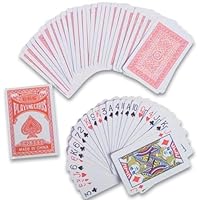A deck of playing cards has 52 different cards (if we remove the Jokers). I draw a card at random from that deck. What is the probability that the card will be the Queen of Diamonds?

The answer is a fraction. Type the numerator in the first box. Type the denominator in the second box. Then click the button. /

The Law of Large Numbers

If a trial (such a play of a game of chance) is repeated many times, then the more times the trial is repeated, the more likely it is that the frequency of any particular event will be close to the probability of that event. For example, if we flip a fair coin many times, the more times we flip it, the more likely it is that the number of "heads" divided by the total number of tosses will be close to 1/2. This may be taken as the definition of probability, or it can be taken as a theorem, in which case it is called the Law of Large Numbers.

Evaluating a game of chance

A casino with a roulette wheel will typically pay "1 to 1" if you bet that a red number will come up and a red number does come up. "1 to 1" means that if you win they give you an amount of money equal to what you bet. If you bet $1 and win, you get to keep your original $1, plus they give you $1 more. If a black or green number comes up, you lose your $1 to the casino.

To figure out whether this kind of gamble is likely to make you money, you can use the concept of expected value.

Expected Value

The expected value is calculated by taking each outcome and multiplying its value by the probability of that outcome, then adding all the products up.

For the roulette wheel, the expected value of betting $1 on Red at 1-1 odds is:

Red numbers/All numbers 18/38	times	What you get $1	equals	$ 18/38
Black numbers/All numbers 18/38	times	What you get $-1	equals	$-18/38
0 and 00/All numbers 2/38	times	What you get $-1	equals	$ -2/38
			Total:	$ -2/38

$18/38 + $-18/38 + $-2/38 = $-2/38, or approximately $-0.0528.

For each $1 you bet, your expected loss (it's a loss because the sign is negative) is just over 5 cents.

Casinos set all of the payoff odds as if the two green zero numbers were not there. Consequently, all roulette bets have the same expectation, $-0.0528 per dollar bet.

For example, if you bet on a single number, the payoff is 35 to 1, as if there were 35 losing numbers and 1 winning number. Really, though, there are 37 losing numbers, so your expected value is:
1/38 times $35 (for when you win), plus
37/38 times $-1 (for when you lose),
which equals ($35 - $37)/38 = $-2/38.

This is how the casino makes money, even though the wheel itself is fair, in the sense that the casino doesn't manipulate it to make you lose. The wheel is fair, but the game is not.

European roulette wheels ("roulette" is from the French for small ball) have a 0 but no 00. Your expected loss over there would be €-0.027 per Euro bet.

A Fair Game

A fair game has an expected value of $0. Roulette in America has an expected value of $-0.0528, approximately, so it's not "fair" in this sense.

The casino could make roulette fair by adjusting the payoffs. For example, if betting on red or black and winning paid 20 to 18, rather than 1 to 1, then the game would be fair. Paying 20 to 18 would mean that if you bet $1 and won, the casino would give you about $1.11. Your expected value would then be:
18/38 times $20/18 (for when your color comes up), plus
18/38 times $-1 (for when the other color comes up), plus
2/38 times $-1 (for when green comes up),
which equals ($20 - $18 - $2)/38 = $0/38 = $0.

There is an analogus concept for insurance: The actuarially fair premium is the premium that exactly equals the expected insurance payoff.

The Expected Value and the Law of Large Numbers

If you go into a casino with $10 and start betting $1 at a time at roulette, sooner or later you'll lose all your $10. Why is this? If your expected loss per $1 bet is $-0.0528, shouldn't you expect to lose just $0.528 when you bet $10?

Choose the better explanation for why you lose all of your money:
I am unlucky. If I go in with $10, on average, I should come out with $10 minus $0.528.
If I keep betting, the total I have bet is more than $10. I bet the same dollars over and over.

The more times you play, the more likely it is that
your net gain will be close to the game's expected value times the total amount that you have bet.

If the game's expected value is less than 0, then what I called a "gain" in that sentence will really be a loss.

We can illustrate this with a roulette simulation.

Roulette Simulation

Below, after this explanation, is a roulette simulation. Before you try it, let me tell you how it works and what it is supposed to show.

We will pretend that we are playing roulette. We will bet on Odd. This means we will win when the little ball on the roulette wheel lands on an odd number. We lose if the ball finishes on an even number. We also lose if the ball finishes on 0 or 00 because, in roulette, 0 and 00 are neither even nor odd.

There is no little ball or wheel inside this computer, of course. Instead, we use a random number generator to simulate spins of the wheet.

If we bet on Odd, there are 18 numbers that win for us: 1, 3, 5, 7, 9, and so forth, up through 35. Twenty numbers lose for us: 2, 4, 6, 8, and so forth through 36, plus 0 and 00, which are neither even nor odd in roulette. Winning pays 1-1, meaning that we get $1 if we win and lose $1 if we don't. Our expected loss per bet is (18-20)/38 = $-0.0528 per dollar bet. The law of large numbers implies that, the more times we spin, the closer we should get to $-0.0528 per dollar bet.

The number that last came up
How many times we won	0
How many times we lost	0
Our net gain (minus means loss)	0
Total bets	0
Gain per dollar bet

If you spin once, you will either win or lose. Your net gain per dollar bet will be either 1 or -1.

If you press the spin 10 button several times, your net gain per dollar bet will vary, but it won't go nearly all the way to 1 or -1.

If you press the spin 1000 button several times, your net gain per dollar bet will vary, but not by nearly as much as for spinning 10 times.

If you press the spin 1 million button several times, the net gain per dollar spent will come out between -0.510 and -0.0540 almost every time. Suppose a roulette wheel in a casino gets two bets every thirty seconds, 12 hours a day. The casino is very likely to make between $51,000 and $54,000 on that roulette wheel.

The more spins, the smaller is the bracket around -2/38.

To further test your understanding of probability concepts, I have another roulette simulation. This one has the bettor use a doubling system, a sure fire way to beat the odds? (This simulation uses a Java applet.)

Evaluating Securities

The application of this roulette model to evaluating financial securities is almost straightforward.

I say "almost" is because of the important phenomenon of risk aversion. A risk averse person is one who is willing to pay money to avoid taking a risk. We discuss that in detail another interactive tutorial. (This is a link, but I recommend working through the rest of this tutorial first.) Leaving risk aversion aside, the application of the roulette model is straightforward.

Suppose you have the opportunity to buy a treasury bill from some country.

A treasury bill is a simple I.O.U., a promise to pay a certain amount of money at a certain time. A typical treasury bill might promise to pay $10,000 in one year. When you buy such a treasury bill, you are lending money, in effect. You give the country some money today. The country promises to give you $10,000 in a year.

If there is no risk that the country won't pay off the bill, then the value of the bill today depends on the current interest rate on no-risk loans. Investors considering buying the bill will offer an amount of money that is less than $10,000. They will offer at most the amount of money $X such that $X would grow to $10,000 in one year if invested in some other no-risk loan. In other words, the investor will offer the present value of a sure $10,000 one year from now.

Let's say that the current interest rate on short-term treasury securities is 2% per year. For this no-risk treasury bill, you would offer at most the amount of money $X such that $X times 1.02 equals $10,000.

We can write this equation: X times 1.02 = 10000. Divide both sides by 1.02 to get X = 10000/1.02 = $9803.92. (For more on this type of calculation, see the interactive tutorial on discounting future income.)

This is why it is said that treasury bills sell "at a discount." You get the 2% interest by giving the treasury an amount that is less than the face value or future value. You give the treasury $9803.92 now. A year from now, they will give you $10,000. You will have earned 2% interest.

Now let's suppose that another country is also selling $10,000 one-year treasury bills. This country's finances are shaky. You estimate that the probability is 90% that the country will actually pay the $10,000 when the year is up. There is a 10% probability that it will pay $0.

Let us calculate the expected present value of that risky treasury bill.

We can start with the present value if there were no risk. It is, $9803.92, if the interest rate on no-risk loans is 2%.

Let us say that there are two possibilities:

The bond will pay $10,000 in one year.
The bond will pay $0 in one year.

From the paragraph above, we have that the probability of paying in full is 90%, and that the probability of paying nothing is 10%.

90% + 10% = 100%, so there are no other possible outcomes.

Place the decimal forms of 90% and 10% in the table below. In other words, type 0.9 and 0.1 in the boxes below. The only thing to figure out is which number goes in which box.

Outcome	Present value of payoff	Probability of outcome
The bond will pay $10,000 next year.	$9803.92
The bond will pay $0 next year.	$0.00

Leaving some space you have the right numbers above.

⇑

For this example, I posited the probability that the country would pay off the bill. How would you make that judgement in practice?

Some economists argue that the market can tell us what the probabilities are. By comparing a security's market price with the market price of a bond that will surely be paid off, one can calculate what the market "thinks" the probability of default is.

We can show how this is supposed to work by turning our current example around.

Suppose one-year $10,000 treasury bills issued by the U.S. (and therefore sure to pay off [if you ignore the crazy wing of the Republican party]) are selling for $9803,92. Country X's one-year $10,000 treasury bills are selling for $8823.53. What does the market think is the probability that Country X will actually pay?

We run the calculation above backwards.

8823.53/9803.92 = 0.9

The market says that the probability of Country X failing is 0.9 or 90%.

That doesn't really answer the question of you should set the probability. If you are deciding how to invest your money, or your institution's money, or your city's money, you have make your own judgement. Hopefully, you won't wind up in jail like the former Jefferson County, Alabama, County Commission President. His county went broke in 2008 after he invested county money in what the market thought were low-risk bond swaps.

This example shows the basics. It could be made more realistic by adding more possible outcomes than just paying in full or paying nothing, such as partial payment or deferred payment. The same method works: List the possibilities, calculate what each is worth today, and multiply each worth by your best guess of the probability of that happening.

In July 2011, the European Union announced a deal that amounted to a controlled partial default for Greece. Greek bonds would be paid at 80% of their face value. For example, a bank that had lent 1,000,000 Euros to Greece will get 800,000 Euros, plus interest payments based on $800,000 rather than $1,000,000. Greek bonds went up in price after the announcement. They had been selling at a discount that was greater than 20%.

By the way, in 2008, as the banks got scared and stopped lending money, some cable news commentators said that investors had gotten "risk averse," and that is why risky securities lose market value. This is not what risk averse means. What happened in 1998 and 2008 and some years in between was that investors changed their assessment of how big the risks were. You may have a certain attitude about gambling on a security with a 90% probability of paying off. Some news event may cause you to think that the probability of paying off has dropped to 50%. Your attitude toward a 90%-sure bet doesn't necessarily change. What changes is that the security no longer offers a 90%-sure bet. So the price you would pay for that security will be much lower, even without any change in your attitude toward risk, which is what risk aversion is about. More about that in the next tutorial.

Effective Interest Rates Vary According to Risk

In the example above, Country X is, in effect, paying a higher interest rate because its bills are risky. The interest it is paying can be calculated like this:

That's much more than the 2% that the sure-bet country is paying. Riskier borrowers have to pay higher interest rates. That's the main reason why, for example, on January 13, 1999, 6-month US Government bonds were paying interest at an annual rate of about 4½%, RJR Nabisco Corporation bonds were paying about 8%, and Argentine telephone company bonds were paying about 11%.

A dramatic example of changing the assessment of risk happened during August 2007. Starting around 2002, banks and similar financial institutions took home mortgages, assembled them into groups, and then sold them to investors. What the banks were selling was the right to collect homeowners' payments on their mortgages.

S&P risk rating	Bonds
AAA	United States	Investment grade
AA+	South Carolina U.S. since Aug. 2011
AA	Citigroup
AA-	Goldman Sachs
A+	Italy
A	AT&T
A-	Malaysia
BBB+	Bulgaria Palmetto Health Alliance
BBB	Sprint-Nextel
BBB-	Whole Foods
BB+	Colombia	Junk
BB	Harrah's
BB-	Indonesia
B	Ford Motor
B-	Six Flags
CCC+	Movie Gallery
CCC	Ecuador
CCC- CC C
D	defaulted

Source: Wall Street Journal, 8/15/2007, p. A10.

The material after this paragraph was written a few years ago. I'm thinking now that the interest rate differences are a better measure of risk than the ratings from the ratings comanies. See this chart, from Nate Silver's blog, which shows how poorly the ratings correlate with the risk of default. For this chart, the measure of risk, on the Y-axis, is how much you have to pay to buy insurance that will pay you if the country defaults. See also The Activist Ratings Agencies and Their Poor Public Sector Predictions. In particular, when the credit raters downgraded U.S. debt in August 2011, the interest rates that the U.S. was paying did not go up.

Assessing the risk of these mortgage-backed securities was a job for ratings firms, particularly Moody's Investors Service and Standard & Poor's. These are well-established companies that have been in the ratings business for many years. (Here is a link to John Moody's 1904 book about why monopolies -- then the darlings of Wall Street but the bane of Progressives -- were good things, in Moody's view. Hmm ... they haven't changed much! )

Moody's and Standard & Poor's have alphanumeric designations for different levels of risk. The chart to the right shows the Standard & Poor's categories with some examples. Borrowers high on that list, like the United States Treasury, are considered low risk. These borrowers pay the lowest interest rates. Interest rates are higher for borrowers lower on the list. As of August 2007, the best junk bonds (BB+) pay about 4½ percentage points more than the best investment grade bonds. The differences can change, though. According to the Wall Street Journal, August 20, 2007, the difference between what A borrowers pay and what the U.S. Treasury pays widened from about ¼ percentage point in July to more than 2 percentage points in mid-August. Ordinarily, the value of a bond depends on the expected value of its future payments. That is what this tutorial teaches. The widening interest difference between AAA and A bonds from July to August 2007 suggested that something else was going on: Investors were panicking. They were avoiding buying corporations' bonds because other investors were doing the same, and the investors were afraid that they would not be able to resell the bonds if they bought them. One day, the demand for commercial paper -- corporations' I.O.U.s -- almost disappeared. Sales of commercial paper that usually took an hour were taking most of the day. It was like a stampede. If you are in the middle of one, you have no choice but to run with the crowd. This was scary, because a corporation that cannot "roll over" its bonds is in the same mess as a homeowner who has a balloon payment due and cannot refinance. Central banks in Europe and the U.S. stopped the stampede by loaning money at lowered interest rates to banks that bought corporate bonds. That seems to have partly worked. Commercial paper is getting bought and sold, but the interest rate spread is still high.

(Some commentators wonder why governments could not similarly encourage bridge loans to hard-pressed homeowners. That is a topic for another place!)

The mortgages in the mortgaged-backed securities were risky to various degrees, depending on such things as how big the down payment was, what the income of the homebuyer family was, and how much credit card or other debt the family was carrying. "Prime" mortgages are home loans with big down payments to families with enough income to meet standards and little or no other debt. "Sub-prime" mortgages are home loans with looser requirements. There are lots of gradations of risk within the sub-prime category. Standard & Poors, Moody's, and other rating companies reviewed the mortgages and estimated, based on recent experience, the probability that each mortgage would be paid. Banks bundled higher probability mortgages together and sold them as packages -- mortage-backed securities -- to investors. Standard & Poor's and other raters gave these securities investment-grade ratings (see table). Those securities could be sold to pension funds and other institutions looking for good returns with low risk. Meantime, the low-probability mortgages were bundled into junk-rated securities. Those went to buyers able and willing to take more risk.

In ordinary times, this can work fine. It did work, up until mid-2006. Homeowners occasionally fall behind on their mortgages for individual reasons, like job loss, divorce, or expensive medical care. These independent random events were expected. Pooling mortgages into groups spreads risk, just like insurance, and the higher interest rates on the riskier securities covered the losses, just as insurance premiums ordinarily do.

Then the housing bubble started to deflate. Banks and mortgage companies had been lending to riskier and riskier people to buy houses. By late 2006, this was backfiring. A growing number of homebuyers were failing to make even their first mortgage payment. Banks pulled back on making risky new loans. This reduced the flow of homebuyers. House prices stopped rising, and started falling in some areas. Homeowners who were counting on refinancing their mortgages could not do so, because they could not get a new mortgage loan as big as the old one. Their houses were not worth as much. Defaults were no longer independent events. Lots of homebuyers were defaulting at once, being stuck with loans that they could not refinance and houses that they could not sell except at a loss.

Ratings companies realized that the past experience that they had been using to assess risk no longer applied. In March 2007, Standard & Poor's was predicting that housing prices would be flat in 2007 and then rise in 2008. By July 2007, Standard & Poor's was predicting an 8% fall in housing prices into early 2008. That month, Moody's and Standard & Poor's lowered the ratings on about a thousand securities that were based on sub-prime mortgage loans. Big international investors got worried about lending money to financial corporations that were counting on income from these mortgage-backed securities. Then the big investors got worried that other big investors were worried about lending to financial corporations held a lot of mortgage-backed securities. No one wants to be the last person to lend money to a loser. That sparked the panic described above.

The ratings companies defend their risk-assessment methodology. They say that they are used to being blamed when things go sour.

The financial crash and interest rates

In mid-September, 2008, after the U.S. Government declined to bail out the failing Lehman Brothers investment bank, the perceived difference in risk between the U.S. Teasury and big banks widened considerably. On one morning (Sept. 18), the "TED" spread, which is the difference between the interest rate on three-month U.S. Treasury bills (3-month I.O.U.'s) and the London Interbank Offered Rate (what big banks charge other big banks for overnight loans), jumped to 3 percentage points. In calmer times (like March 2008), the interest rate diffence was about 1/4 of a percentage point. Banks with spare cash flocked to U.S. Treasury bills, driving the interest rate on 3-month bills down on 0.05%. No, that is not a typographical error. Banks were so eager to lend their money to a safe borrower that the U.S. was borrowing at an interest rate of 1/20th of a percent. Lending among banks was almost nil, until the U.S. and other governments announced measures to pump money into the world's banking system. In the U.S., those measures included the TARP program.

Review

A fair game is a game that ...
... is not rigged. The every number on the roulette wheel, or every card in the deck, has an equal chance of being selected or dealt.
... has an expected payoff value of $0.

Obamacare is requiring health insurance companies to pay out -- for health care -- at least 85% of their premiums. Does this make health insurance a fair bet?
Yes, fair.
No, not fair.

If investors think that the probability has gone up that a certain security will not pay off, what happens to the price of the security?
The price should go down.
The price should go up.
The price should not change.

Why do we need to distinguish risk from undercertainty?
We don't. A statistical analysis of the past will tell you what you need to know about the future.
We do. Risk is about probabilities. Probabilities can change.

Regarding that last answer, see http://baselinescenario.com/2013/08/28/regulators-repeat-exactly-what-they-did-during-the-last-housing-boom/

Thanks for participating! The follow-up tutorial is about risk aversion.

August 28, 2013