Introductory Probability and Statistics Review
This page goes over some basic probability and statistics concepts that you got in BIOS
700.
Probability
The probability of an event is a fraction between 0 and 1.
1 is the probability of an event that is sure to happen. The probability
that the sun will rise tomorrow is 1.
0 is the probability of an event that cannot happen. The probability
that a Bridge hand will contain a Joker is 0, because Bridge is played with a deck from which the Jokers have been removed.
Here's how you get probabilities between 0 and 1: Suppose there are
a number of equally likely events. Some events represent a "win"
and some a "loss." The probability of winning is the number of winning
events divided by the total number of events. Such well-defined situations
arise in practice only in games.
For example, consider a coin with a "heads" side and a "tails"
side. If we assume that the two sides are equally likely to be up when
the coin is tossed and lands on a table, then the probability of "heads"
is 1/2 and the probability of "tails" is 1/2.
For another example, an American roulette wheel has 38 spaces. Each
space has a number and a color. Eighteen of the spaces are red. Eighteen
are black. Two are green. If you bet that the ball will fall in a red space,
your probability of winning is 18/38.
Your turn:
A deck of playing cards has 52 different cards, if we remove the Jokers. I draw a card at random from that deck. What is the probability that the card will be the Queen of Diamonds?
For your answer, you can type two numbers with a slash / sign in between to indicate division. Alternatively, you can type in a decimal number.
The Law of Large Numbers
If a trial (such a play of a game of chance) is repeated many times, then
the more times the trial is repeated, the more likely it is that the frequency
of any particular event will be close to the probability of that event.
For example, if we flip our coin many times, the more times we flip it,
the more likely it is that the the number of "heads" divided by the total
number of tosses will be close to 1/2. This may be taken as the definition
of probability, or it can be taken as a theorem, in which case it is called
the Law of Large Numbers.
Law of Large Numbers Example
This applet simulates tossing a coin over and over again. Click Start to start the coin tosses. This same button restarts the tosses if you stop them with the Stop button. Click Faster to reduce the delay time between simulated tosses.
This coin, simulated by a random number generator, has two sides that are equally likely to come up.
If you let this run, the proportion of heads in the number of tosses will approach one-half (0.5). Rarely will the proportion be exactly 1/2. Instead, it will fluctuate around 0.5, with the fluctuations slowly getting smaller.
Statistics
A statistic is a number calculated from numerical data. An example
of a statistic is the mean.
Mean
The mean of a list of numbers is calculated by adding all the numbers
up, then dividing by how many numbers there are. The mean is also called
the "average."
Some examples:
-
Consider a coin that has a "0" painted on one side and a "1" on the other
side. The mean of the numbers on the coin is (0+1) / 2, which is 1/2.
-
Consider a die, a cube with the numbers 1 through 6 on its sides. The mean
of the numbers on the die is (1+2+3+4+5+6) / 6 = 21 / 6 = 3.5.
Your turn:
What is the mean of these numbers: 1, 1, 2, 8?
The mean is a measure of central tendency. The mean height of 21-year-old
men in the U.S. is 177 cm, or 5' 10". The mean height of women here is
164 cm, or 5' 4". This tells us that, in the U.S., men are generally taller
than women. It does not imply that every man is taller than every woman.
Expected Value
Suppose have a game of chance with a numerical outcome.
For example, we can flip our coin painted with "0" and "1" and see which
number comes up. The expected value is calculated by taking
each outcome and multiplying its value by the probability of that outcome,
then adding all the products up.
For the coin, the expected value is:
(0 times the probability of 0) + (1 times the probability of 1).
If the coin is fair, so that the two sides are equally likely to come
up, then the expected value is:
(0 times 1/2) + (1 times 1/2) = 0 + 1/2 = 1/2.
If all outcomes are equally likely, then the expected value will equal
the mean of all the outcomes.
Suppose we flip our coin many times, and calculate the mean of all the
outcomes of the tosses. The more flips we do, the more likely it
is that the mean of all the accumulated outcomes will be close to the expected
value. The simulation above does this. If you say that a head is worth 1
and a tail is worth 0, the "proportion of heads" fraction is the mean of all the outcomes so far.
It does tend to get closer and closer to 0.5.
Variance
The variance measures how spread out a list of numbers is, how much
the numbers differ from their mean. To calculate the variance:
General instructions
for calculating a variance: |
For example, suppose you have
a coin with 0 and 1 painted on its sides: |
| Take each data item. |
The data items are 0 and 1. |
| Subtract the mean from each. |
Subtract the mean ( 1/2 ) from each: -1/2 and 1/2 |
| Square each. |
Square each: 1/4 and 1/4 |
| Add them all up |
Add them all up: 1/4 + 1/4 = 1/2 |
Divide by the number of data items
to get the variance. |
Divide 1/2 by the number of data items ( 2 ), to get 1/4.
The variance is 1/4. |
Your turn:
What is the variance of these numbers: 3, 3, 3, 3. (Yes, the four numbers are the same.)
This one is harder:
What is the variance of 1, 1, 2, 8?
Notice that 3, 3, 3, 3 and 1, 1, 2, 8 have the same mean but different variances.
If you were designing a system for handling eggs,
you would want to know the both mean and the variance of the size of the eggs.
Standard Deviation
The standard deviation is the square root of the variance. Like
the variance, the standard deviation measures spread. The variance involves
squaring the data numbers. Taking the square root of the variance gives
you a number that is in the same units as the original data. This allows
for an intuitive interpretation of the standard deviation: Usually, depending
on the shape of the distribution (see next), about 2/3 of the data numbers
are within one standard deviation of the mean.
Distributions
If the outcome numbers are discreet, meaning that there is a certain number
of possible outcomes, then the distribution is a list of all possible
outcomes and each one's probability.
If the outcome numbers are continuous, meaning that the outcome could
be any number in either a finite range or an infinite range, then you can't
list all possible outcomes and each one's probability. What you can do
instead is give a mathematical formula that would tell you, for any given
x
, what the probability is that the outcome will be less than x .
This is the distribution function. Distributions are often visualized
using the density function. On a graph of the density function,
if you pick any two possible outcome values on the x axis, and draw
vertical lines at those values up from the
x axis to where they
intersect the density function's curve, then you will have an enclosed
area with straight sides, a straight botton, and a curved top. The size
of that area tells you the probability that the outcome will be between
the two x values.
For example, a distribution we'll be using often this semester is the
normal
distrbution. Its density function is "the bell curve."

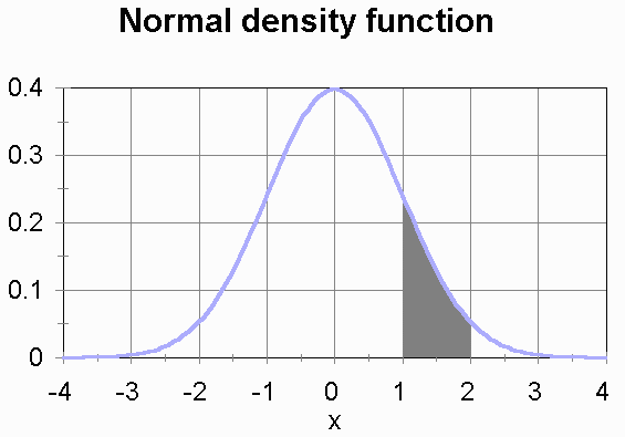
This is the density function for a normal distribution with a mean
of 0 and a standard deviation of 1. The density function is constructed
so that the total area under the curve is 1. (The area under the curve
is unbounded, because the curve goes off forever in both directions without
ever quite touching the x axis, but even so the area under the curve
is finite and equal to 1.) The area of the shaded region is the probability
of a outcome number between 1 and 2.
Algebraic Expressions with Summation Signs
For these expressions, the data items are represented as:

There are N data items.
For our coin with a 0 on one side and a 1 on the other, the
data items are x1 = 0 and x2 = 1. N = 2.
Mean
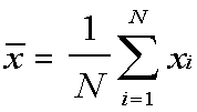
The mean is represented by x with a line over it, read "x bar."

A shorter notation for this uses the summation sign, the capital sigma:

This means:
-
Substitute 1 for the i in the expression to the right of the big
sigma. This gives you the first data item.
-
Keep substitutimg successive numbers for i until you have substituted
N
for i. This gives you the second through the Nth data item.
-
Add all those terms up.
-
Divide the sum by N.
This is read, "X-bar equals one over N times the sum, from i equals 1 to
N, of x-sub-i."
The course readings use this notation often. If it seems intimidating,
take the time to work through what the expression means. Proceed methodically
and you can do it.
Variance
The variance is:

You can read a formula like this from the inside out:
-
Take a data item (xi).
-
Subtract the mean from it ( - x-bar).
-
Square the difference (the 2 exponent outside the parentheses).
-
Do the same for the 1st through the Nth data item (the i=1 below the Sigma and the N above it).
-
Add them all up (what the Sigma means).
-
Divide the sum by the number of data items (the 1/N in front).
Standard Deviation
The standard deviation is the square root of the variance.

The views and opinions expressed in this page are strictly those of
the page author. The contents of this page have not been reviewed or approved
by the University of South Carolina.
E-mail:


